BandNorm-tutorial
BandNorm-tutorial.RmdIntroduction
The advent of single-cell sequencing technologies in profiling 3D genome organization led to development of single-cell high-throughput chromatin conformation (scHi-C) assays. Data from these assays enhance our ability to study dynamic chromatin architecture and the impact of spatial genome interactions on cell regulation at an unprecedented resolution. At the individual cell resolution, heterogeneity driven by the stochastic nature of chromatin fiber, various nuclear processes, and unwanted variation due to sequencing depths and batch effects poses major analytical challenges for inferring single cell-level 3D genome organizations.
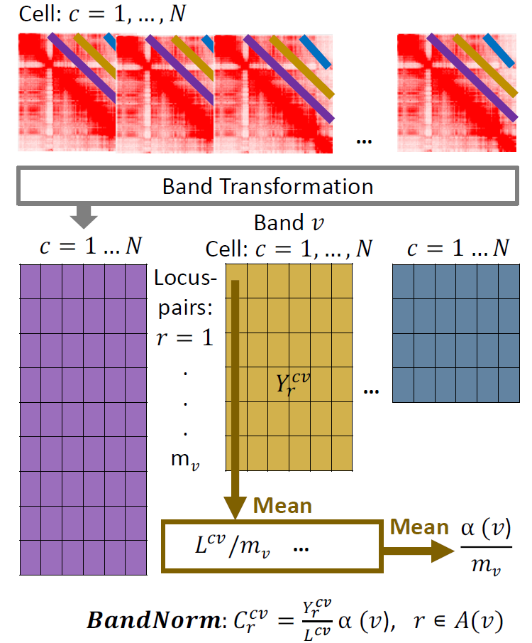
To explicitly capture chromatin conformation features and distinguish cells based on their 3D genome organizations, we develop a simple and fast band normalization approach, BandNorm. BandNorm first removes genomic distance bias within a cell, and sequencing depth normalizes between cells. Consequently, BandNorm adds back a common band-dependent contact decay profile for the contact matrices across cells. The former step is achieved by dividing the interaction frequencies of each band within a cell with the cell’s band mean. The latter step is implemented by multiplying each scaled band by the average band mean across cells.
Installation
To use BandNorm, the following packages are necessary:
install.packages(c('ggplot2', 'dplyr', 'data.table', 'Rtsne', 'umap'))

if (!requireNamespace("devtools", quietly=TRUE))
    install.packages("devtools")

devtools::install_github("immunogenomics/harmony")
BandNorm can be installed from Github:
devtools::install_github('sshen82/BandNorm', build_vignettes = FALSE)Also, if the user doesn’t have default R path writing permission, it is possible to install the package to the personal library:
withr::with_libpaths("personalLibraryPath", devtools::install_github("sshen82/BandNorm"))Format of input
There are three possible ways to input the data:
- A path containing all cells in the form of [chr1, binA, chr2, binB, count], the cell looks like below:
chr1    0       chr1    1000000 9
chr1    1000000 chr1    1000000 200
chr1    0       chr1    2000000 2
chr1    1000000 chr1    2000000 4
chr1    2000000 chr1    2000000 220
chr1    1000000 chr1    3000000 1
chr1    2000000 chr1    3000000 11
chr1    3000000 chr1    3000000 197
chr1    1000000 chr1    4000000 1
chr1 2000000 chr1 4000000 2- An R data.frame in the form of [chr1, binA, binB, count, diag, cell_name]. The column names should be c(“chrom”, “binA”, “binB”, “count”, “diag”, “cell”). Below we print the example data.
library(BandNorm)
#> Loading required package: ggplot2
#> Warning: package 'ggplot2' was built under R version 4.0.5
#> Loading required package: dplyr
#>
#> Attaching package: 'dplyr'
#> The following objects are masked from 'package:stats':
#>
#>     filter, lag
#> The following objects are masked from 'package:base':
#>
#>     intersect, setdiff, setequal, union
#> Loading required package: data.table
#> Warning: package 'data.table' was built under R version 4.0.5
#>
#> Attaching package: 'data.table'
#> The following objects are masked from 'package:dplyr':
#>
#>     between, first, last
#> Loading required package: Rtsne
#> Warning: package 'Rtsne' was built under R version 4.0.5
#> Loading required package: umap
#> Warning: package 'umap' was built under R version 4.0.5
#> Loading required package: progress
#> Warning: package 'progress' was built under R version 4.0.4
#> Loading required package: harmony
#> Loading required package: Rcpp
#> Warning: package 'Rcpp' was built under R version 4.0.5
#> Loading required package: Matrix
#> Warning: package 'Matrix' was built under R version 4.0.5
#> Loading required package: gmodels
#> Warning: package 'gmodels' was built under R version 4.0.4
#> Loading required package: furrr
#> Warning: package 'furrr' was built under R version 4.0.5
#> Loading required package: future
#> Loading required package: matrixStats
#> Warning: package 'matrixStats' was built under R version 4.0.5
#>
#> Attaching package: 'matrixStats'
#> The following object is masked from 'package:dplyr':
#>
#>     count
#> Loading required package: Seurat
#> Warning: package 'Seurat' was built under R version 4.0.5
#> Attaching SeuratObject
#> Loading required package: strawr
#> Warning: package 'strawr' was built under R version 4.0.5
#> Loading required package: rmarkdown
#>
#> Attaching package: 'rmarkdown'
#> The following object is masked from 'package:future':
#>
#>     run
#> Loading required package: viridis
#> Warning: package 'viridis' was built under R version 4.0.5
#> Loading required package: viridisLite
#> Warning: package 'viridisLite' was built under R version 4.0.5
#> Loading required package: sparsesvd
#> Warning: package 'sparsesvd' was built under R version 4.0.5
#> Loading required package: GenomicInteractions
#> Loading required package: InteractionSet
#> Warning: package 'InteractionSet' was built under R version 4.0.5
#> Loading required package: GenomicRanges
#> Warning: package 'GenomicRanges' was built under R version 4.0.3
#> Loading required package: stats4
#> Loading required package: BiocGenerics
#> Warning: package 'BiocGenerics' was built under R version 4.0.5
#> Loading required package: parallel
#>
#> Attaching package: 'BiocGenerics'
#> The following objects are masked from 'package:parallel':
#>
#>     clusterApply, clusterApplyLB, clusterCall, clusterEvalQ,
#>     clusterExport, clusterMap, parApply, parCapply, parLapply,
#>     parLapplyLB, parRapply, parSapply, parSapplyLB
#> The following objects are masked from 'package:dplyr':
#>
#>     combine, intersect, setdiff, union
#> The following objects are masked from 'package:stats':
#>
#>     IQR, mad, sd, var, xtabs
#> The following objects are masked from 'package:base':
#>
#>     anyDuplicated, append, as.data.frame, basename, cbind, colnames,
#>     dirname, do.call, duplicated, eval, evalq, Filter, Find, get, grep,
#>     grepl, intersect, is.unsorted, lapply, Map, mapply, match, mget,
#>     order, paste, pmax, pmax.int, pmin, pmin.int, Position, rank,
#>     rbind, Reduce, rownames, sapply, setdiff, sort, table, tapply,
#>     union, unique, unsplit, which.max, which.min
#> Loading required package: S4Vectors
#> Warning: package 'S4Vectors' was built under R version 4.0.3
#>
#> Attaching package: 'S4Vectors'
#> The following object is masked from 'package:future':
#>
#>     values
#> The following object is masked from 'package:Matrix':
#>
#>     expand
#> The following objects are masked from 'package:data.table':
#>
#>     first, second
#> The following objects are masked from 'package:dplyr':
#>
#>     first, rename
#> The following object is masked from 'package:base':
#>
#>     expand.grid
#> Loading required package: IRanges
#> Warning: package 'IRanges' was built under R version 4.0.3
#>
#> Attaching package: 'IRanges'
#> The following object is masked from 'package:data.table':
#>
#>     shift
#> The following objects are masked from 'package:dplyr':
#>
#>     collapse, desc, slice
#> The following object is masked from 'package:grDevices':
#>
#>     windows
#> Loading required package: GenomeInfoDb
#> Warning: package 'GenomeInfoDb' was built under R version 4.0.5
#> Loading required package: SummarizedExperiment
#> Warning: package 'SummarizedExperiment' was built under R version 4.0.3
#> Loading required package: MatrixGenerics
#> Warning: package 'MatrixGenerics' was built under R version 4.0.3
#>
#> Attaching package: 'MatrixGenerics'
#> The following objects are masked from 'package:matrixStats':
#>
#>     colAlls, colAnyNAs, colAnys, colAvgsPerRowSet, colCollapse,
#>     colCounts, colCummaxs, colCummins, colCumprods, colCumsums,
#>     colDiffs, colIQRDiffs, colIQRs, colLogSumExps, colMadDiffs,
#>     colMads, colMaxs, colMeans2, colMedians, colMins, colOrderStats,
#>     colProds, colQuantiles, colRanges, colRanks, colSdDiffs, colSds,
#>     colSums2, colTabulates, colVarDiffs, colVars, colWeightedMads,
#>     colWeightedMeans, colWeightedMedians, colWeightedSds,
#>     colWeightedVars, rowAlls, rowAnyNAs, rowAnys, rowAvgsPerColSet,
#>     rowCollapse, rowCounts, rowCummaxs, rowCummins, rowCumprods,
#>     rowCumsums, rowDiffs, rowIQRDiffs, rowIQRs, rowLogSumExps,
#>     rowMadDiffs, rowMads, rowMaxs, rowMeans2, rowMedians, rowMins,
#>     rowOrderStats, rowProds, rowQuantiles, rowRanges, rowRanks,
#>     rowSdDiffs, rowSds, rowSums2, rowTabulates, rowVarDiffs, rowVars,
#>     rowWeightedMads, rowWeightedMeans, rowWeightedMedians,
#>     rowWeightedSds, rowWeightedVars
#> Loading required package: Biobase
#> Warning: package 'Biobase' was built under R version 4.0.3
#> Welcome to Bioconductor
#>
#>     Vignettes contain introductory material; view with
#>     'browseVignettes()'. To cite Bioconductor, see
#>     'citation("Biobase")', and for packages 'citation("pkgname")'.
#>
#> Attaching package: 'Biobase'
#> The following object is masked from 'package:MatrixGenerics':
#>
#>     rowMedians
#> The following objects are masked from 'package:matrixStats':
#>
#>     anyMissing, rowMedians
#>
#> Attaching package: 'SummarizedExperiment'
#> The following object is masked from 'package:SeuratObject':
#>
#>     Assays
#> The following object is masked from 'package:Seurat':
#>
#>     Assays
data(hic_df)
print(hic_df[1:10, ])
#>    chrom  binA  binB count  diag    cell
#> 1   chr1 0e+00 0e+00    38 0e+00 Astro_1
#> 2   chr1 0e+00 1e+06     1 1e+06 Astro_1
#> 3   chr1 1e+06 1e+06   105 0e+00 Astro_1
#> 4   chr1 1e+06 2e+06     1 1e+06 Astro_1
#> 5   chr1 2e+06 2e+06   116 0e+00 Astro_1
#> 6   chr1 2e+06 3e+06     2 1e+06 Astro_1
#> 7   chr1 3e+06 3e+06   133 0e+00 Astro_1
#> 8   chr1 3e+06 4e+06     1 1e+06 Astro_1
#> 9   chr1 4e+06 4e+06   112 0e+00 Astro_1
#> 10 chr1 3e+06 5e+06 1 2e+06 Astro_1- We also support using Juicer .hic format, and you can use bandnorm_juicer function to run it. We will have a thorough example for this in the future.
For the example dataset, we also have batch information and cell-type information. Note that the cell_name in those external information should be consistent with the hic_df file.
data(batch)
data(cell_type)
print(batch[1:10, ])
#>       cell_name  batch
#>  [1,] "Astro_1"  "181218_21yr"
#>  [2,] "Astro_2"  "181218_21yr"
#>  [3,] "Astro_3"  "181218_21yr"
#>  [4,] "Astro_4"  "181218_21yr"
#>  [5,] "Astro_5"  "181218_21yr"
#>  [6,] "Astro_6"  "181218_21yr"
#>  [7,] "Astro_7"  "181218_21yr"
#>  [8,] "Astro_8"  "181218_21yr"
#>  [9,] "Astro_9"  "181218_21yr"
#> [10,] "Astro_10" "181218_21yr"
print(cell_type[1:10, ])
#>       cell_name  cluster
#>  [1,] "Astro_1"  "Astro"
#>  [2,] "Astro_2"  "Astro"
#>  [3,] "Astro_3"  "Astro"
#>  [4,] "Astro_4"  "Astro"
#>  [5,] "Astro_5"  "Astro"
#>  [6,] "Astro_6"  "Astro"
#>  [7,] "Astro_7"  "Astro"
#>  [8,] "Astro_8"  "Astro"
#>  [9,] "Astro_9"  "Astro"
#> [10,] "Astro_10" "Astro"
Download existing single-cell Hi-C data
You can also use download_schic function to download real data. The available data includes Kim2020, Li2019, Ramani2017, and Lee2019. You can specify one of the cell-types in those cell lines. There are also summary files available for them, and the summary includes batch, cell-type, depth and sparsity information. You can go to this website for more information. We won’t run it here since it will mess up your computer.
# download_schic("Li2019", cell_type = "2i", cell_path = getwd(), summary_path = getwd())Use BandNorm
We provide a demo scHi-C data named hic_df, sampled 400 cells of Astro, ODC, MG, Sst, four cell types and chromosome 1 from Ecker2019 for test run. After obtaining the hic_df file, you can use the bandnorm function to normalize the data. The result consists of 6 columns: chromosome, binA, binB, diag (which is binB - binA), cell (which is the name of the cell), and BandNorm. You can use the save option to save the normalized file, and if so, you need to give a path for output.
bandnorm_result = bandnorm(hic_df = hic_df, save = FALSE)
bandnorm_result[1:10, ]
#>    chrom  binA  binB  diag    cell   BandNorm
#> 1   chr1 0e+00 0e+00 0e+00 Astro_1 120.131557
#> 2   chr1 0e+00 1e+06 1e+06 Astro_1   8.051104
#> 3   chr1 1e+06 1e+06 0e+00 Astro_1 331.942461
#> 4   chr1 1e+06 2e+06 1e+06 Astro_1   8.051104
#> 5   chr1 2e+06 2e+06 0e+00 Astro_1 366.717385
#> 6   chr1 2e+06 3e+06 1e+06 Astro_1  16.102209
#> 7   chr1 3e+06 3e+06 0e+00 Astro_1 420.460450
#> 8   chr1 3e+06 4e+06 1e+06 Astro_1   8.051104
#> 9   chr1 4e+06 4e+06 0e+00 Astro_1 354.071958
#> 10  chr1 3e+06 5e+06 2e+06 Astro_1   8.392744
# bandnorm_result = bandnorm(hic_df = hic_df, save = TRUE, save_path = getwd())
Then, you can use create_embedding function to obtain a PCA embedding for the data. You can choose to use Harmony to remove the batch effect.
embedding = create_embedding(hic_df = bandnorm_result, do_harmony = TRUE, batch = batch, chrs = "chr1")
#> Harmony 1/10
#> Harmony 2/10
#> Harmony 3/10
#> Harmony converged after 3 iterations
embedding[1:10, ]
#> [,1] [,2] [,3] [,4] [,5] [,6]
#> Astro_1 260.4890 8.767428 -38.15255 -24.67058474 41.438432 42.359819
#> Astro_2 257.7442 -2.951022 -45.12881 0.09234945 16.898551 12.308446
#> Astro_3 263.3217 -9.622970 -15.05707 -1.82768494 9.421532 -10.324896
#> Astro_4 257.4937 -3.686170 -38.18991 -30.22117139 15.970829 14.971427
#> Astro_5 253.8995 -21.326499 -19.08085 -23.88545629 17.700467 28.380758
#> Astro_6 255.1843 7.330198 -28.17633 -25.69458359 2.444970 7.701229
#> Astro_7 263.1543 15.709052 -33.01460 -12.05113123 9.612310 5.296989
#> Astro_8 261.5342 -5.386315 -46.78872 -4.27357902 9.024755 5.942738
#> Astro_9 258.5931 -5.285896 -20.20657 -20.84444116 19.050879 14.885779
#> Astro_10 262.5704 1.565764 -19.03290 -19.23823636 6.431833 28.061190
#> [,7] [,8] [,9] [,10] [,11] [,12]
#> Astro_1 27.375286 2.595551 -56.6927552 42.0278246 -6.64794030 -30.997075
#> Astro_2 -7.319173 9.577958 -7.8033543 11.7208199 14.06890106 -17.897096
#> Astro_3 21.925646 23.086416 15.7495192 4.5084385 4.84878002 -7.029905
#> Astro_4 19.614074 -3.310085 0.4682037 4.1700977 -14.10580821 3.919195
#> Astro_5 25.013790 -2.860101 1.1129512 44.3856683 16.67119525 -94.647483
#> Astro_6 -11.077577 17.896088 -6.4499603 0.2569391 0.02233005 -1.287126
#> Astro_7 6.238411 9.604235 -2.1418579 -4.8596355 -9.75191614 9.259222
#> Astro_8 -12.830410 24.374966 13.1372461 -2.2591202 1.57709507 -21.180022
#> Astro_9 -2.931585 -15.193808 35.2331178 47.2257586 12.91352783 -44.113965
#> Astro_10 6.369004 -5.737758 -6.0984339 31.5061841 -17.83135495 -7.297526
#> [,13] [,14] [,15] [,16] [,17] [,18]
#> Astro_1 24.8389123 48.014163 22.594232 26.879686 -17.764963 47.575686
#> Astro_2 26.7372741 7.112525 -2.100140 -9.758681 9.129671 -22.321543
#> Astro_3 6.3331554 23.932153 -3.554945 1.070171 13.202461 10.333723
#> Astro_4 15.7940490 1.013382 -4.964899 -19.919792 -4.115079 -2.493478
#> Astro_5 44.1986970 31.957885 -50.658311 5.041710 28.953036 -11.821712
#> Astro_6 46.1472793 35.984804 4.290632 3.137027 -18.789369 -1.698368
#> Astro_7 7.4893642 26.285780 4.960351 -12.157652 1.855262 9.015391
#> Astro_8 0.2081309 -3.852817 39.317673 -8.172145 -20.812369 -10.652579
#> Astro_9 77.9487476 -25.929523 22.183102 32.192150 47.480473 -24.668663
#> Astro_10 32.6119878 26.130073 27.947224 -13.650015 -2.480721 16.657205
#> [,19] [,20] [,21] [,22] [,23]
#> Astro_1 -52.165887 -44.77027195 -33.5171701 174.2001968 72.226768
#> Astro_2 -17.111597 0.03440498 2.4519609 -6.7115828 -8.946803
#> Astro_3 -6.104868 -34.79714807 -16.9931502 5.4223607 10.766928
#> Astro_4 1.602215 10.69226879 -16.4557316 -10.8021012 -7.617040
#> Astro_5 13.968589 -117.71146709 -21.4002871 -102.4880111 8.550867
#> Astro_6 -11.901826 27.62252463 7.5348045 -3.4529971 50.485852
#> Astro_7 -22.520698 8.27432244 0.3743479 3.3861833 17.936365
#> Astro_8 -6.182087 6.40240844 20.1300829 39.9619402 -28.535149
#> Astro_9 -50.749904 88.50609366 55.8169814 -22.5412733 -61.490664
#> Astro_10 -24.548488 11.99957044 11.7413168 0.8271987 -18.653642
#> [,24] [,25] [,26] [,27] [,28] [,29]
#> Astro_1 -16.386022 -54.869325 20.560727 81.544077 -13.76737 -153.072692
#> Astro_2 7.268235 1.832398 -2.904150 -7.814636 5.43311 -1.038148
#> Astro_3 7.664850 -8.364236 10.543454 -16.986662 33.25000 12.957056
#> Astro_4 25.398605 -17.013670 3.492867 -11.492420 -19.42296 18.991759
#> Astro_5 -147.772999 -122.943107 54.735317 -50.354511 69.00397 81.567382
#> Astro_6 15.977662 12.425930 4.278786 -2.759817 -31.24299 -10.258419
#> Astro_7 28.127373 -6.674850 36.518524 -11.394666 -23.13568 11.706313
#> Astro_8 28.649519 35.369948 14.517941 -1.017830 40.95661 25.122970
#> Astro_9 -67.940815 -13.220251 21.377759 186.058095 16.48910 82.722282
#> Astro_10 12.763440 3.186854 -42.558798 -1.472243 -17.96547 2.968344
#> [,30] [,31] [,32] [,33] [,34] [,35]
#> Astro_1 9.590189 42.816171 25.5879791 82.152135 -17.152270 26.9323154
#> Astro_2 -6.171868 -11.269152 -0.7524294 2.601524 -12.055115 -12.9924918
#> Astro_3 35.840878 -2.266545 17.6956974 21.980148 76.642959 7.4629514
#> Astro_4 7.619683 15.392685 -18.2376936 -12.042492 4.811808 -15.5632095
#> Astro_5 -63.368410 -10.478491 -6.9576844 9.294764 -5.968970 54.9452854
#> Astro_6 30.374323 3.745559 -7.5131172 -52.411802 -19.763387 -2.1776394
#> Astro_7 18.674288 28.937264 -26.4556766 3.266864 34.270544 -0.3702734
#> Astro_8 13.131849 38.719632 16.2648726 -5.324021 -56.595264 18.6355156
#> Astro_9 -19.637507 10.015595 68.1805446 27.492296 -1.892617 21.1763405
#> Astro_10 19.153321 6.796307 -43.1824271 -51.727511 23.113677 -29.6471542
#> [,36] [,37] [,38] [,39] [,40] [,41]
#> Astro_1 73.577289 -76.6473786 -10.249177 -11.69798 -53.204571 9.6541863
#> Astro_2 -9.541354 3.6128059 -7.283889 28.27541 -8.976800 -0.5436889
#> Astro_3 5.760162 0.9157821 15.045677 61.58504 2.394746 27.5026545
#> Astro_4 22.436398 22.8350392 25.681786 -27.13307 -38.641330 -3.7815305
#> Astro_5 68.409064 21.0722508 4.983493 -31.11380 -20.931421 43.3814474
#> Astro_6 21.957560 24.7474594 12.136265 38.14670 -43.547662 -39.2408240
#> Astro_7 -56.278708 3.4877407 20.064065 44.00578 36.069266 -9.1911690
#> Astro_8 62.941845 30.2315027 -36.536162 -119.47765 -11.550092 15.4002350
#> Astro_9 -59.620860 -22.9745626 -6.709363 76.00778 69.084106 -25.9574979
#> Astro_10 13.663266 24.7698930 -14.476287 -23.14196 52.038852 65.3056339
#> [,42] [,43] [,44] [,45] [,46] [,47]
#> Astro_1 1.4042453 -8.010776 -9.936818 10.086427 34.95841 -6.878220
#> Astro_2 9.9176614 -30.112688 33.152526 -2.607484 -10.06566 26.102611
#> Astro_3 -11.2904710 -5.961986 -3.732932 -39.483373 39.32086 -13.379015
#> Astro_4 47.6176604 15.884958 23.432234 -3.734371 16.84145 -56.400890
#> Astro_5 -77.8378575 -15.213299 -21.548621 -6.503176 -11.15840 9.462415
#> Astro_6 12.6594503 -32.945805 -41.975947 -14.210205 -51.50516 -13.824187
#> Astro_7 -30.9920359 39.241872 -11.385210 13.075889 13.05906 71.223717
#> Astro_8 0.7003749 24.847937 50.955284 -29.392734 -54.54864 -35.502715
#> Astro_9 8.4094760 -25.572851 -22.823801 10.015358 34.10033 -27.521115
#> Astro_10 35.8006038 -23.976404 23.721624 -22.409581 14.47883 1.179911
#> [,48] [,49] [,50]
#> Astro_1 27.144996 -19.977632 41.7302522
#> Astro_2 9.757486 9.627174 -18.2998709
#> Astro_3 -51.163939 -84.691785 -2.2715623
#> Astro_4 -34.260223 -1.579583 37.4665829
#> Astro_5 52.559095 2.943192 -3.6451595
#> Astro_6 48.168772 -17.226910 -15.7795729
#> Astro_7 9.193921 -22.290690 0.2038873
#> Astro_8 -33.839609 38.958284 21.1158886
#> Astro_9 -33.060039 54.412258 51.1445118
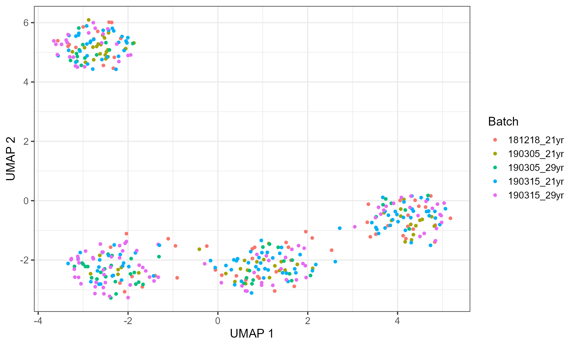
#> Astro_10 54.534217 15.884740 -65.5443043Finally, using the embedding, you can use UMAP or tSNE to get a projection of all the cells on the 2D plane. If you have the cell-type information or batch information, it is possible to color them on the plot.
plot_embedding(embedding, "UMAP", cell_info = cell_type, label = "Cell Type")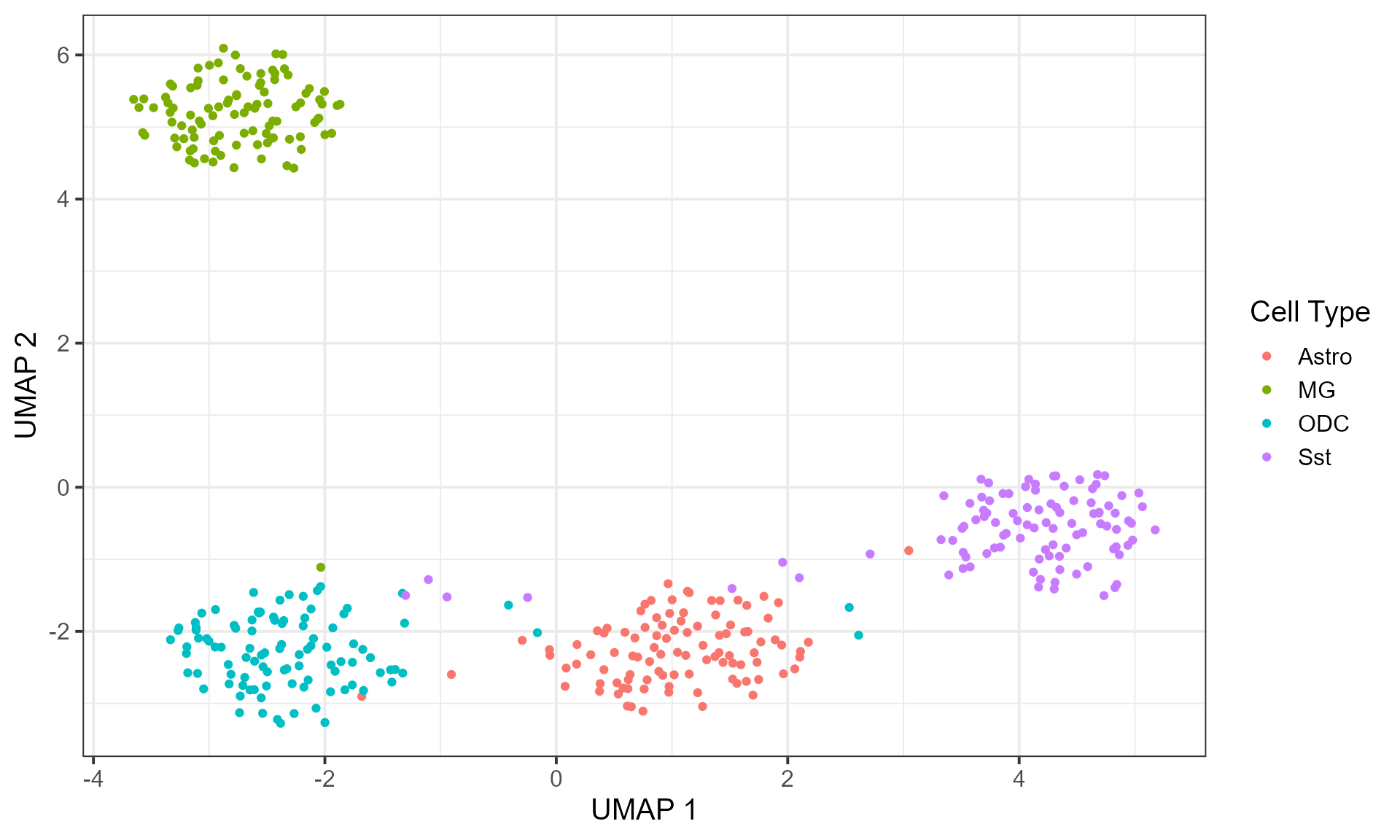
plot_embedding(embedding, "UMAP", cell_info = batch, label = "Batch")