scGAD-tutorial
scGAD-tutorial.RmdIntroduction
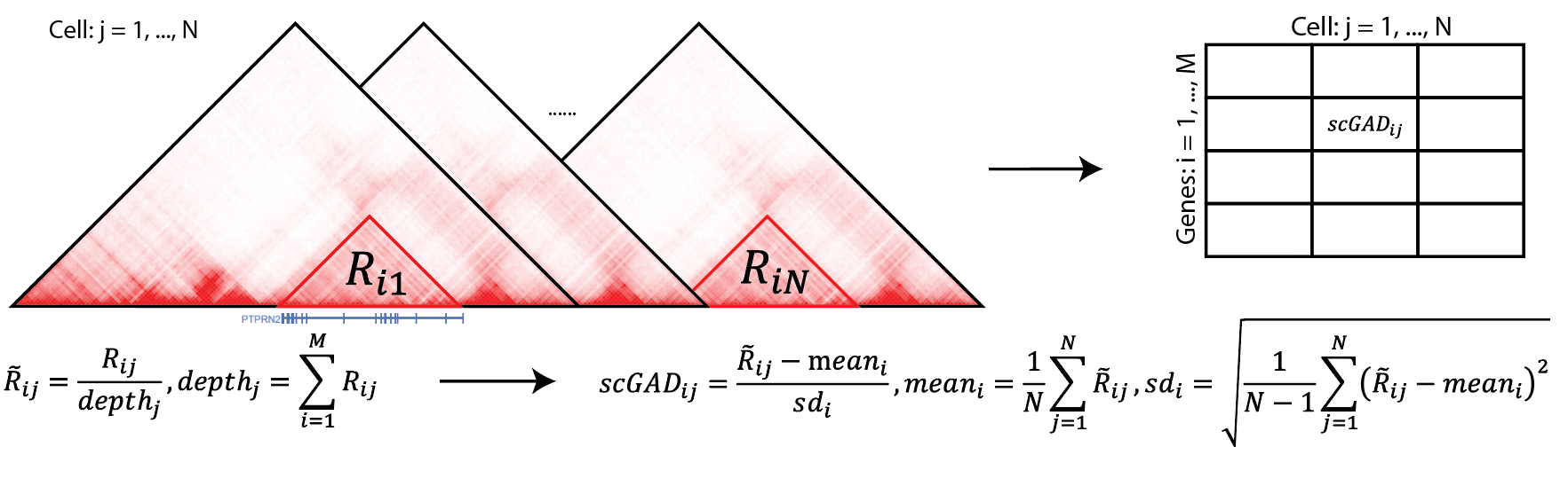
Recent advancements in single-cell technologies enabled the profiling of 3D genome structures in a single-cell fashion. Quantitative tools are needed to fully leverage the unprecedented resolution of single-cell high-throughput chromatin conformation (scHi-C) data and integrate it with other single-cell data modalities. We present single-cell gene associating domain (scGAD) scores as a dimension reduction and exploratory analysis tool for scHi-C data. scGAD enables summarization at the gene level while accounting for inherent gene-level genomic biases. Low-dimensional projections with scGAD capture clustering of cells based on their 3D structures. scGAD enables identifying genes with significant chromatin interactions within and between cell types. We further show that scGAD facilitates the integration of scHi-C data with other single-cell data modalities by enabling its projection onto reference low-dimensional embeddings of scRNA-seq. Please refer to our manuscript, scGAD: single-cell gene associating domain scores for exploratory analysis of scHi-C data, on BioRxiv for the comprehensive study of scGAD.
In this tutorial, we will walk you through
- The usage of scGAD function to convert single-cell Hi-C contact matrices into gene x cell scGAD score matrix.
- Integration of scGAD scores of scHi-C with scRNA-seq reference panel.
Installation
Please refer to the BandNorm R package installation section in BandNorm tutorial. scGAD is one of the key functions of BandNorm R package.
1. scGAD Usage
1.1 Format of input scHi-C data
scGAD function allows two formats of input data. It can be A. the path to the input data or B. a data.frame object containing all the interaction from all the cells with cell name in each row.
A. A path to the folder where the single-cell Hi-C contact matrices are saved. One file per cell in the form of 5-columns bed file, namely chrA, binA, chrB, binB, count:
chr1    0       chr1    10000 9
chr1    10000   chr1    10000 20
chr1    0       chr1    20000 2
chr1    10000   chr1    20000 4
chr1    20000   chr1    20000 22
chr1    10000   chr1    30000 1
chr1    20000   chr1    30000 11
chr1    30000   chr1    30000 197
chr1    10000   chr1    40000 1
chr1    20000   chr1    40000 2
B. Another way is to provide a data.frame object which includes all interactions information plus the cell name where such interactions occur. The data frame should have 5 columns and look like chrom, binA, binB, count, cell. The column names in here should be exactly the same as stated, and the order of columns doesn’t matter. Option B is not recommended for the large volumne of single-cell Hi-C data set especially when it is implemented with limited computational resources like laptop. However, it can be fast if it is run on servers or computers which have sufficient memory to store such large data.frame object.
> scgad_df
chrom   binA    binB    count   cell
chr1    0       10000   9       cell_1
chr1    10000   10000   20      cell_1
chr1    0       20000   2       cell_1
chr1    10000   20000   4       cell_1
chr1    20000   20000   22      cell_1
chr1    10000   30000   1       cell_2
chr1    20000   30000   11      cell_2
chr1    30000   30000   197     cell_2
chr1    10000   40000   1       cell_2
chr1    20000   40000   2       cell_3
1.2 Format of input gene coordinate file.
you can get mm9, mm10, hg19 and hg38 using data(Annotations). Below is the first ten rows of mm9Annotations. The first column is chromosome, s1 and s2 are start and end of the gene, the fourth column is the strand, and the last column is the gene name.
> mm9Annotations
chr      s1      s2 strand gene_name
chr1 3195982 3661579      -      Xkr4
chr1 4334224 4350473      -       Rp1
chr1 4481009 4486494      -     Sox17
chr1 4763287 4775820      -    Mrpl15
chr1 4797869 4876851      +    Lypla1
   ---
chry 2086590 2097768      +   Rbmy1a1
chry 2118049 2129045      +   Gm10256
chry 2156899 2168120      +   Gm10352
chry 2390390 2398856      +    Gm3376
chry 2550262 2552957      +    Gm3395
1.3 Demo run of scGAD
The demo data used for illustrations was generated based on the real scHi-C data from Tan et al. 2021. Cell. 350 cells were randomly sampled from three cell types, Mature Oligodendrocyte, Microglia Etc. and Hippocampal Granule Cell. The aim of the demo data is to show the format of input object to scGAD function and how to run scGAD function to get the scGAD scores.
library(BandNorm)
#> Loading required package: ggplot2
#> Warning: package 'ggplot2' was built under R version 4.0.5
#> Loading required package: dplyr
#> Warning: package 'dplyr' was built under R version 4.0.5
#>
#> Attaching package: 'dplyr'
#> The following objects are masked from 'package:stats':
#>
#>     filter, lag
#> The following objects are masked from 'package:base':
#>
#>     intersect, setdiff, setequal, union
#> Loading required package: data.table
#> Warning: package 'data.table' was built under R version 4.0.4
#>
#> Attaching package: 'data.table'
#> The following objects are masked from 'package:dplyr':
#>
#>     between, first, last
#> Loading required package: Rtsne
#> Warning: package 'Rtsne' was built under R version 4.0.3
#> Loading required package: umap
#> Warning: package 'umap' was built under R version 4.0.3
#> Loading required package: progress
#> Warning: package 'progress' was built under R version 4.0.4
#> Loading required package: harmony
#> Loading required package: Rcpp
#> Warning: package 'Rcpp' was built under R version 4.0.5
#> Loading required package: Matrix
#> Warning: package 'Matrix' was built under R version 4.0.5
#> Loading required package: gmodels
#> Warning: package 'gmodels' was built under R version 4.0.4
#> Loading required package: doParallel
#> Warning: package 'doParallel' was built under R version 4.0.3
#> Loading required package: foreach
#> Warning: package 'foreach' was built under R version 4.0.3
#> Loading required package: iterators
#> Warning: package 'iterators' was built under R version 4.0.3
#> Loading required package: parallel
#> Loading required package: matrixStats
#> Warning: package 'matrixStats' was built under R version 4.0.3
#>
#> Attaching package: 'matrixStats'
#> The following object is masked from 'package:dplyr':
#>
#>     count
#> Loading required package: Seurat
#> Warning: package 'Seurat' was built under R version 4.0.5
#> Attaching SeuratObject
#> Loading required package: strawr
#> Warning: package 'strawr' was built under R version 4.0.5
#> Loading required package: rmarkdown
#> Warning: package 'rmarkdown' was built under R version 4.0.5
library(curl)
#> Warning: package 'curl' was built under R version 4.0.5
#> Using libcurl 7.64.1 with Schannel
h = new_handle(dirlistonly=TRUE)
con = curl("http://ftp.cs.wisc.edu/pub/users/kelesgroup/siqi/scGAD/scGADExample.rda", "r", h)
load(con)
close(con)

gad_score = scGAD(hic_df = scgad_df, genes = geneANNO, depthNorm = TRUE)
After using scGAD function, you can get the scGAD score like below:
>gad_score
        cell_1    cell_2    cell_3
Xkr4    -2.29     -0.87     -0.29
Rp1     0.42      0.09      -1.93
Rgs20   -0.14     -1.25     0.16
1.4 Parallel running
In scGAD, we also allows for parallel running for scGAD with parameter cores and threads. In here, cores means number of CPUs used, and each CPU focuses on one particular cell during the iteration. If cores = 4, then the scGAD score for four cells can be simutaneously calculated. threads also indicates number of CPUs, but this is used specifically for fread function in data.table. By default, data.table will likely to overload your CPUs, so it is important to manually set this number. It is recommended to set threads so that threads * cores is smaller than the total number of CPUs.
gad_score = scGAD(hic_df = scgad_df, genes = geneANNO, depthNorm = TRUE, cores = 4, threads = 12)1.5 Visualizion of the lower-dimension representation of scGAD
Then, you can use PCA to first perform dimensionality-reduction, and choose the first two principal components to visualize the result, and cells are clearly separated.
library(ggplot2)
summary = summary[match(colnames(gad_score), summary$cell), ]
gadPCA = prcomp(gad_score)$rotation[, 1:15]
gadPCA = data.frame(gadPCA, cellTypes = summary$`cell-type cluster`)
ggplot(gadPCA, aes(x = PC1, y = PC2, col = cellTypes)) + geom_point() + theme_bw(base_size = 20) + scale_color_manual(breaks = c("Hippocampal Granule Cell", "Mature Oligodendrocyte", "Microglia Etc."),
                   values = c("#1B4F72", "#F39C12", "#000000"))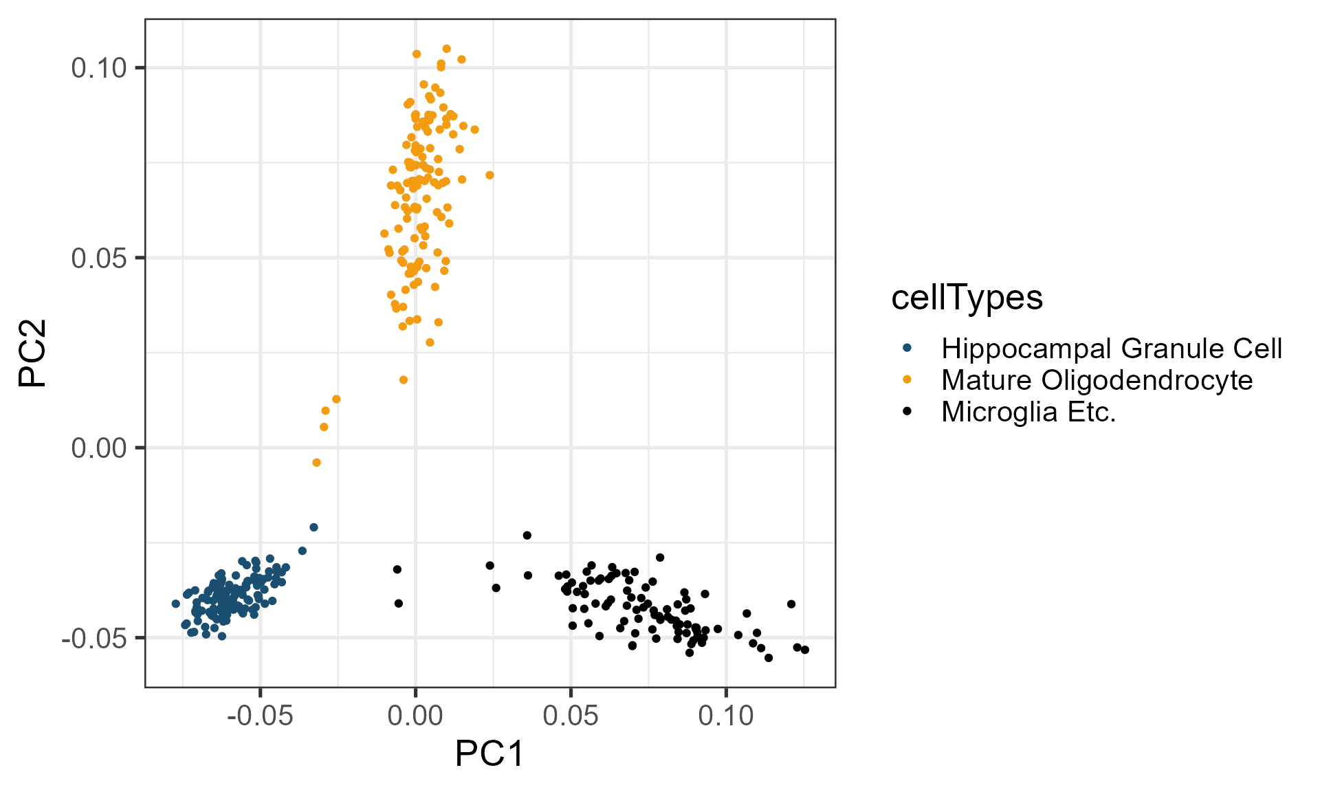
2. Projection of scGAD on scRNA-seq
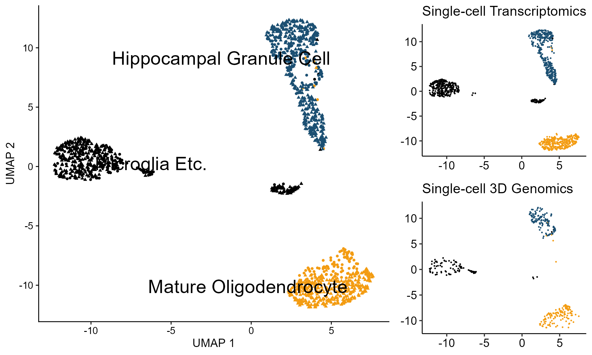
Finally, with scRNA-seq data on hand, we can do projection from scGAD to scRNA-seq. For scRNA-seq, we have 1076 cells from Mature Oligodendrocyte, Microglia Etc. and Hippocampal Granule Cell. These cells are also from Tan et al. 2021. Cell.
library(ggplot2)
library(viridis)
#> Warning: package 'viridis' was built under R version 4.0.5
#> Loading required package: viridisLite
#> Warning: package 'viridisLite' was built under R version 4.0.5
library(dplyr)
library(gridExtra)
#>
#> Attaching package: 'gridExtra'
#> The following object is masked from 'package:dplyr':
#>
#>     combine
library(ggpubr)
#> Warning: package 'ggpubr' was built under R version 4.0.3
library(Seurat)

DataList = list(scGAD = gad_score, scRNAseq = RNA)
cellTypeList = list(scGAD = summary$`cell-type cluster`, scRNAseq = cellTypeRNA)
names(cellTypeList[[1]]) = summary$cell
names(cellTypeList[[2]]) = colnames(RNA)

combinedAssay = runProjection(DataList, doNorm = c(FALSE, FALSE), cellTypeList)
#> Warning: The following arguments are not used: row.names
#> Warning: The following arguments are not used: row.names
#> Scaling features for provided objects
#> Finding all pairwise anchors
#> Running CCA
#> Merging objects
#> Finding neighborhoods
#> Finding anchors
#>  Found 1722 anchors
#> Filtering anchors
#>  Retained 541 anchors
#> Merging dataset 1 into 2
#> Extracting anchors for merged samples
#> Finding integration vectors
#> Finding integration vector weights
#> Integrating data
#> Warning: The default method for RunUMAP has changed from calling Python UMAP via reticulate to the R-native UWOT using the cosine metric
#> To use Python UMAP via reticulate, set umap.method to 'umap-learn' and metric to 'correlation'
#> This message will be shown once per session
#> 17:22:03 UMAP embedding parameters a = 0.9922 b = 1.112
#> 17:22:03 Read 1426 rows and found 5 numeric columns
#> 17:22:03 Using Annoy for neighbor search, n_neighbors = 30
#> 17:22:03 Building Annoy index with metric = cosine, n_trees = 50
#> 0%   10   20   30   40   50   60   70   80   90   100%
#> [----|----|----|----|----|----|----|----|----|----|
#> **************************************************|
#> 17:22:03 Writing NN index file to temp file C:\Users\solei\AppData\Local\Temp\RtmpAB56FU\file246825161fc1
#> 17:22:03 Searching Annoy index using 1 thread, search_k = 3000
#> 17:22:03 Annoy recall = 100%
#> 17:22:03 Commencing smooth kNN distance calibration using 1 thread
#> 17:22:04 Initializing from normalized Laplacian + noise
#> 17:22:04 Commencing optimization for 500 epochs, with 55294 positive edges
#> 17:22:07 Optimization finished

p_celltype <- DimPlot(combinedAssay, reduction = "umap", label = TRUE, repel = TRUE, pt.size = 1.3, shape.by = "method", label.size = 8) +
xlab("UMAP 1") +
ylab("UMAP 2") +
scale_color_manual(breaks = c("Hippocampal Granule Cell", "Mature Oligodendrocyte", "Microglia Etc."),
                   values = c("#1B4F72", "#F39C12", "#000000")) +
rremove("legend")


pRNA = combinedAssay@reductions$umap@cell.embeddings %>% data.frame %>% mutate(celltype = c(cellTypeList[[1]], cellTypeList[[2]]), label = c(rep("scGAD", length(cellTypeList[[1]])), rep("scRNA-seq", length(cellTypeList[[2]])))) %>%
filter(label == "scRNA-seq") %>%
ggplot(aes(x = UMAP_1, y = UMAP_2, color = celltype)) +
geom_point(size = 0.3) +
theme_pubr(base_size = 14) +
scale_color_manual(breaks = c("Hippocampal Granule Cell", "Mature Oligodendrocyte", "Microglia Etc."),
                   values = c("#1B4F72", "#F39C12", "#000000")) +
xlab("UMAP 1") +
ylab("UMAP 2") +
rremove("legend") +
ggtitle("Single-cell Transcriptomics") + theme(axis.title = element_blank())


pGAD = combinedAssay@reductions$umap@cell.embeddings %>% data.frame %>% mutate(celltype = c(cellTypeList[[1]], cellTypeList[[2]]), label = c(rep("scGAD", length(cellTypeList[[1]])), rep("scRNA-seq", length(cellTypeList[[2]])))) %>%
filter(label == "scGAD") %>%
ggplot(aes(x = UMAP_1, y = UMAP_2, color = celltype)) +
geom_point(size = 0.3) +
theme_pubr(base_size = 14) +
scale_color_manual(breaks = c("Hippocampal Granule Cell", "Mature Oligodendrocyte", "Microglia Etc."),
                   values = c("#1B4F72", "#F39C12", "#000000")) +
xlab("UMAP 1") +
ylab("UMAP 2") +
rremove("legend") +
ggtitle("Single-cell 3D Genomics") +
 theme(axis.title = element_blank())


lay = rbind(c(1, 1, 2))
grid.arrange(p_celltype, arrangeGrob(pRNA, pGAD, ncol = 1, nrow = 2), layout_matrix = lay)